The JSON Playground in SingleStoreDB

SingleStoreDB’s new playground allows users to run queries over TPC-H, TPC-DS and a semi-structured game dataset sourced from a Confluent Cluster provided by DataGen.

In this post, you will learn how to work with JSON data in SingleStoreDB utilizing the json_game_data dataset in the playground, and get several tips and tricks on schema and query optimizations.  

Explore the SingleStoreDB playground.

Navigate to the Playground

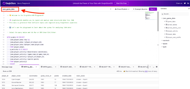
The SingleStoreDB playground allows for reads against the database, and opens with a SQL editor and four pre-loaded databases.

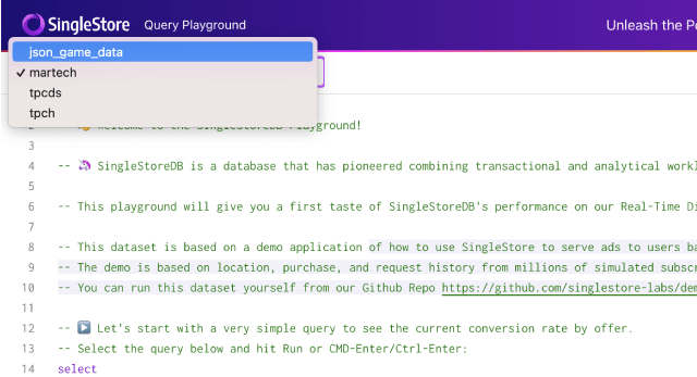
On the top left, click the database drop down and select the json_game_data database.

After the json_game_data is selected, clicking on the example queries button in the top right will open a list of queries that may be loaded directly onto the SQL editor.

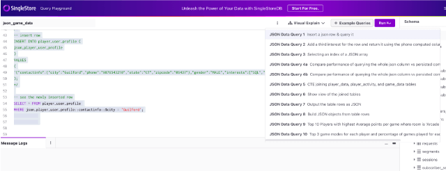
These queries are designed to guide users in quickly learning some best practices on working with JSON in SingleStoreDB.

Tables With JSON Data in SingleStoreDB:

There are four Kafka pipelines ingesting JSON data into the workspace.  

These pipelines are streaming into tables called:

• player_activity
• game_data
• game_data
• player_user_profile

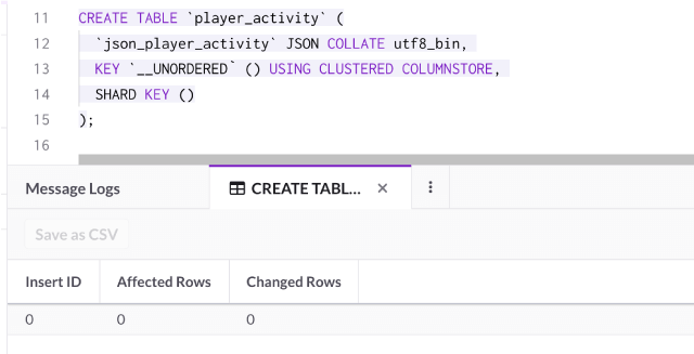
SingleStoreDB natively supports the JSON datatype within the data definition language (DDL).  To create a table with JSON data, simply add the JSON datatype column within the CREATE TABLE statement:

Table with a single JSON column

CREATE TABLE `player_activity` (
 `json_player_activity` JSON COLLATE utf8_bin,
  KEY `__UNORDERED` () USING CLUSTERED COLUMNSTORE,
  SHARD KEY ()
 );  

This is a valid way to bring in the data from the JSON pipeline and queries may be executed against the JSON column without problems, but the entire JSON will be scanned for every query.

Persisted computed columns

In SingleStoreDB, the recommended method of working with JSON is to have a column that stores JSON data, as well as PERSISTED COMPUTED columns on important keys that are frequently joined or filtered.

Creating these columns include setting the column name, the location of the key within the JSON and the persisted data type.

Here is an example of a persisted JSON column:

`game_room_id` as json_player_activity::%game_room_id PERSISTED
BIGINT,

In this case the table definition is as follows:

CREATE TABLE `player_user_profile` (
 `json_player_user_profile` JSON COLLATE utf8_bin,
 `gender` as json_player_user_profile :: $gender PERSISTED longtext
  CHARACTER SET utf8 COLLATE utf8_general_ci,
  `contact_info` as json_player_user_profile :: $contactinfo 
  PERSISTED longtext CHARACTER SET utf8 COLLATE utf8_general_ci,
 `city` as json_player_user_profile :: contactinfo :: $city 
  PERSISTED longtext CHARACTER SET utf8 COLLATE utf8_general_ci,
 `phone` as json_player_user_profile :: contactinfo ::% phone 
  PERSISTED bigint(20),
  `state` as json_player_user_profile :: contactinfo :: $state 
  PERSISTED longtext CHARACTER SET utf8 COLLATE utf8_general_ci,
 `zipcode` as json_player_user_profile :: contactinfo ::% zipcode 
  PERSISTED smallint(6),
  `interests` as json_player_user_profile :: $interests PERSISTED 
  longtext CHARACTER SET utf8 COLLATE utf8_general_ci,
  `interests_1` as json_player_user_profile :: interests :: `0` 
  PERSISTED longtext CHARACTER SET utf8 COLLATE utf8_general_ci,
   `interests_2` as json_player_user_profile :: interests :: `1` 
  PERSISTED longtext CHARACTER SET utf8 COLLATE utf8_general_ci,
   `interests_3` as json_player_user_profile :: interests :: `2` 
  PERSISTED longtext CHARACTER SET utf8 COLLATE utf8_general_ci,
   `regionid` as json_player_user_profile :: $regionid PERSISTED 
  longtext CHARACTER SET utf8 COLLATE utf8_general_ci,
   `registertime` as json_player_user_profile ::% registertime 
  PERSISTED bigint(20),
   `userid` as json_player_user_profile :: $userid PERSISTED longtext 
  CHARACTER SET utf8 COLLATE utf8_general_ci,
   KEY `registertime` (`registertime`) USING CLUSTERED COLUMNSTORE,
   KEY `userid` (`userid`) USING HASH,
   KEY `regionid` (`regionid`) USING HASH,
   KEY `interests` (`interests`) USING HASH,
   KEY `interests_1` (`interests_1`) USING HASH,
   KEY `interests_2` (`interests_2`) USING HASH,
   KEY `interests_3` (`interests_3`) USING HASH,
   SHARD KEY ()
   )
   ;

All other tables were created using similar syntax.

The column with all JSON data

The first column json_player_user_profile is where data is ingested into the Kafka pipeline, and the other columns are parsing the data within separate columns that are used for the shard, sort and hash keys.

The data shape for each rows is as follows:

{
 "contactinfo": {
    "city": "San Carlos",
    "phone": "6502215368",
    "state": "CA",    
    "zipcode": "94070"
  },
   "gender": "OTHER",
   "interests": [
   "Game",
   "Sport" 
  ],   
   "regionid": "Region_4",
   "registertime": 1487715806379,
   "userid": "User_1"
  }  

All other columns are computed from the json_player_user_profile column. 

Grabbing the desired key within the whole JSON column can be done by selecting the json_player_user_profile column, and adding ::  to go to the next level within the JSON.

For example, to get the value for the key “userid” which is on the first level of the JSON, the syntax would be as follows:

json_player_user_profile::$userid

Nested and subsequent JSON levels may be accessed using additional :: syntax after each level

For example to get the nested key of “city” within “contact_info”, the syntax looks like this:

json_player_user_profile::$interests

% and $ symbols

When parsing out the computed columns, the semi-colon notation ::, ::$, and ::% may be used to update JSON objects:

• ::$ will declare the object as a string
• ::% will declare the object as a double

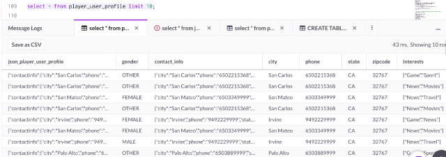
Querying the JSON Tables

As soon as the data streams into SingleStoreDB, it is queryable.Here are the first 10 rows of the player_user_profile table:

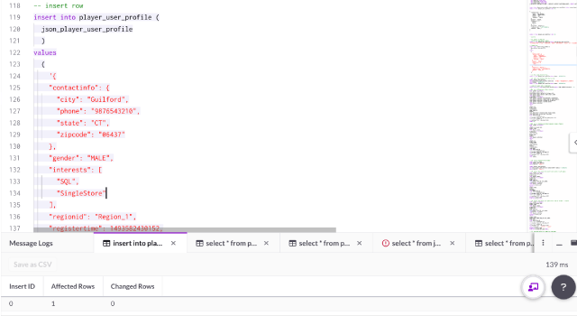
Q1. Insert a JSON row, then find it by city

New JSON rows can be added by inserting into the whole JSON column. In this case the column is json_player_user_profile:

-- insert row
insert into player_user_profile (
 json_player_user_profile
 )
values
 (
   '{"contactinfo":{"city": "Guilford",
     "phone": "9876543210",
     "state": "CT",
     "zipcode": "06437"} ,
   "gender": "MALE",
   "interests": [
     "SQL",
     "SingleStore"
   ],
   "regionid": "Region_1",
   "registertime": 1493582430152,
   "userid": "User_10"} '
 );

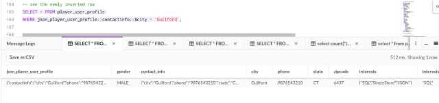
Let’s take a look at the newly inserted row by checking the city name:

SELECT * FROM player_user_profile
WHERE json_player_user_profile::contactinfo::$city = 'Guilford';

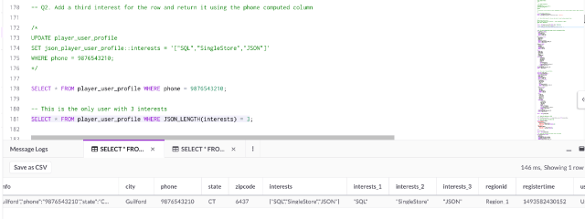
Q2. Update the inserted row and return it using the phone persisted computed column, or the JSON_LEGNTH function

By updating the JSON key within the json_player_user_profile column, persisted computed columns will automatically be updated with the new value.

Here’s an example of adding a new interest “JSON” to our newly created row:

UPDATE player_user_profile
SET json_player_user_profile::interests = 
'["SQL","SingleStore","JSON"]'
WHERE phone = 9876543210;
 
SELECT * FROM player_user_profile WHERE phone = 9876543210;
 
-- This is the only user with 3 interests
SELECT * FROM player_user_profile WHERE JSON_LENGTH(interests) = 3;

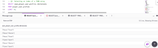
Q3. Selecting an index of a JSON array

Notice the JSON rows in the player_user_profile have a nested JSON array ‘interests’:

SELECT json_player_user_profile::$interests
FROM player_user_profile
LIMIT 10;

Select the index within the array using this syntax:

-- Return the first index of the interests array
SELECT json_player_user_profile::interests::`0`
FROM player_user_profile
LIMIT 10;

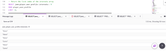
The ::0 syntax after interests is selecting the first index within the interests array. Replace the ‘0’ with ‘1’ to select the second position within the index, and so on.

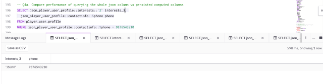
Q4a. Compare performance of querying the whole JSON column vs. persisted computed columns (whole JSON)

The keys have already been parsed into computed columns for the player_user_profile table. These columns eliminate the need to scan the entire JSON for queries that call frequently used keys within the JSON.

For the comparison, the third interest is selected from the new row that has been added with the filter on the phone number ‘9876543210’.

First, the query is run using the whole JSON column ‘json_player_user_profile’:

SELECT json_player_user_profile::interests::`2` interests_3,
 json_player_user_profile::contactinfo::%phone phone
FROM player_user_profile
WHERE json_player_user_profile::contactinfo::%phone = 9876543210;

Using the Visual Profiler, the operations to execute the query (along execution times) are visualized:

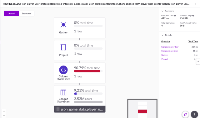
On the summary located in the top right corner, the total execution time is 447ms.

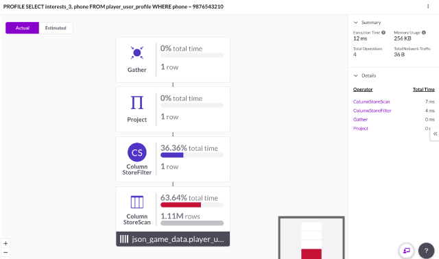
Q4b. Compare performance of querying the whole JSON column vs. persisted computed columns (persisted computed)

The same query as Q4a is run using the persisted computed columns, instead of scanning through the entire JSON column.

SELECT interests_3,
 phone
FROM player_user_profile
WHERE phone = 9876543210;

Using the Visual Profiler, you’ll notice the execution time is only 12ms — a 37.25x improvement for this query!

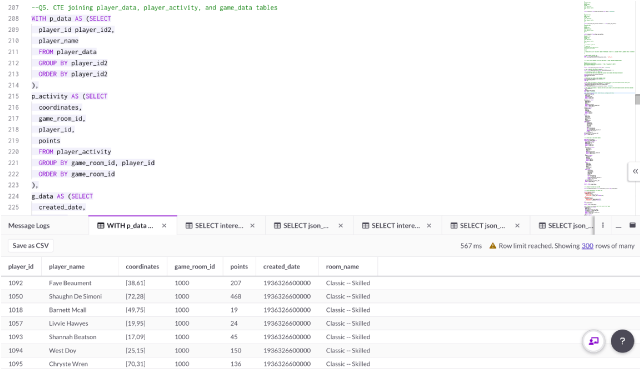
Q5. Joining the player_data, player_activity, and game_data table using Common Table Expressions (CTE)

After exploring the data, it seems that the data within all three of these tables are randomly generated, but there are columns like player_id and game_id that may be joined together.

Let’s create a dataset by joining these tables to use for the next few queries:

WITH p_data AS (SELECT
 player_id player_id2,
 player_name
 FROM player_data
 GROUP BY player_id2
 ORDER BY player_id2
 ),
p_activity AS (SELECT
 coordinates,
 game_room_id,
 player_id,
 points
 FROM player_activity
 GROUP BY game_room_id, player_id
 ORDER BY game_room_id
 ),
g_data AS (SELECT
 created_date,
 game_id,
 room_name
 FROM game_data
 GROUP BY game_id
 ORDER BY game_id
 )
SELECT
 player_id,
 player_name,
 coordinates,
 game_room_id,
 points,
 created_date,
 room_name
FROM (SELECT
     coordinates,
     created_date,
     game_room_id,
     room_name,
     player_id,
     points
     FROM p_activity pa
     LEFT JOIN g_data gd
     ON pa.game_room_id = gd.game_id
     ORDER BY game_room_id
   ) AS pgd
LEFT JOIN p_data pd
ON pgd.player_id = pd.player_id2
ORDER BY game_room_id
;

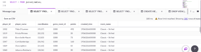
Q6. Show joined tables as a view

The result in Q5 will be used for future queries, so a view of this table called ‘joined_tables’ has been added.

/*
CREATE VIEW joined_tables AS
 WITH p_data AS (SELECT
 player_id player_id2,
 player_name
 FROM player_data
 GROUP BY player_id2
 ORDER BY player_id2
 ),
 p_activity AS (SELECT
   coordinates,
   game_room_id,
   player_id,
   points
   FROM player_activity
   GROUP BY game_room_id, player_id
   ORDER BY game_room_id
 ),
 g_data AS (SELECT
   created_date,
   game_id,
   room_name
   FROM game_data
   GROUP BY game_id
   ORDER BY game_id
 )
 SELECT
   player_id,
   player_name,
   coordinates,
   game_room_id,
   points,
   created_date,
   room_name
FROM (SELECT
       coordinates,
       created_date,
       game_room_id,
       room_name,
       player_id,
       points
       FROM p_activity pa
      LEFT JOIN g_data gd
       ON pa.game_room_id = gd.game_id
       ORDER BY game_room_id
     ) AS pgd
 LEFT JOIN p_data pd
 ON pgd.player_id = pd.player_id2
 ORDER BY game_room_id
;
*/

See the view:

SELECT * FROM joined_tables;

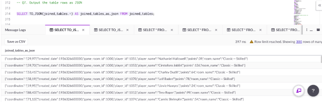
Q7. Output table rows as JSON

SingleStoreDB has several useful functions for working with JSON.  To see the rows from Q6 as JSON, the TO_JSON function may be utilized:

SELECT TO_JSON(joined_tables.*) AS joined_tables_as_json FROM 
joined_tables;

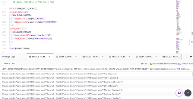
Q8. Build nested JSON objects from columns on your table

Using the joined_tables view, customized JSON objects may be created using the JSON_BUILD_OBJECT function. 

The following example demonstrates creating a nested object that includes player data and game data as well as typecasting values using :>datatype syntax:

SELECT JSON_BUILD_OBJECT(
'player_details',
 JSON_BUILD_OBJECT(
   'player_id', player_id:>INT,
   'player_name', player_name:>VARCHAR(100)
 ),
'game_details',
 JSON_BUILD_OBJECT(
   'game_room_id', game_room_id:>INT,
   'room_name', room_name:>VARCHAR(25)
 )
)
from joined_tables;

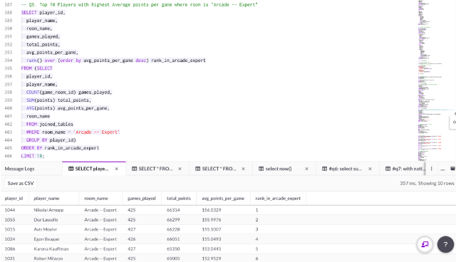
Q9. The top 10 players with the highest average points per game in the room “Arcade — Expert”

Using the joined_tables view, a dataset using three JSON tables is created where analytical queries may be run.

The number of games, total points and average points per game for each player is aggregated with query:

SELECT player_id,
 player_name,
 room_name,
 games_played,
 total_points,
 avg_points_per_game,
 rank() over (order by avg_points_per_game desc) rank_in_arcade_expert
FROM (SELECT
 player_id,
 player_name,
 COUNT(game_room_id) games_played,
 SUM(points) total_points,
 AVG(points) avg_points_per_game,
 room_name
 FROM joined_tables
 WHERE room_name = 'Arcade -- Expert'
 GROUP BY player_id)
ORDER BY rank_in_arcade_expert
LIMIT 10;

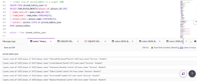
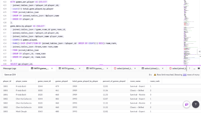
Q10. The top three game modes for each player and percentage of games played in each room from a JSON view

For the final query, a view has been created of the joined_tables in a single JSON column:

CREATE VIEW joined_tables_json AS
SELECT JSON_BUILD_OBJECT('player_id',player_id:>INT,
 'game_room_id', game_room_id:>INT,
 'room_name', room_name:>VARCHAR(25),
 'player_name', player_name:>VARCHAR(25),
 'points', points:>INT) AS joined_tables_json
FROM joined_tables;

The JSON is extracted from the joined_tables_json view, and joining the table with CTE’s allows for robust analytics on our dataset.

WITH games_per_player AS (SELECT
 joined_tables_json::%player_id player_id,
 count(*) total_game_played_by_player
 FROM joined_tables_json
 GROUP BY joined_tables_json::$player_name
 ORDER BY player_id
),
game_data_by_player AS (SELECT
 joined_tables_json::%game_room_id game_room_id,
 joined_tables_json::%player_id player_id,
 joined_tables_json::$player_name player_name,
 COUNT(*) games_played,
 RANK() OVER (PARTITION BY joined_tables_json::%player_id  ORDER BY 
 COUNT(*) DESC) room_rank,
  joined_tables_json::$room_name room_name
  FROM joined_tables_json
  GROUP BY player_id, room_name
  ORDER BY player_id, room_rank
)
SELECT gp.player_id,
 player_name,
 games_played,
 room_name,
 total_game_played_by_player,
 ROUND(games_played/total_game_played_by_player *100,2) 
 percent_of_games_played,
 room_rank
FROM game_data_by_player gp
INNER JOIN games_per_player gpp
ON gp.player_id = gpp.player_id
where room_rank <=3
ORDER BY player_id, percent_of_games_played desc;

In Summary

Working with JSON data in SingleStoreDB is easy and powerful. Using the right strategies outlined here including Persisted Computed Columns, SingleStoreDB JSON functions and schema design decisions may power JSON-intensive applications at scale!

See these queries in action in our new SingleStoreDB Playground.

Try SingleStoreDB free today.