
In 2016, Pandora chose SingleStore to serve as the data store and foundation for solving a specific business problem.
In this post, we explore:
- The Business Problem — what were we trying to solve?
- The Previous System — a few details
- Requirements — business requirements (and a few technical ones too)
- The Contenders — what did the options look like
- About SingleStore
- How We Implemented SingleStore
- Data Strategy: Columnstore vs. Rowstore
- Hardware Details
- Into the Weeds
- Summary
- The Business Problem
The first step in finding a solution is to clearly define the problem. The goal was not to find some way to solve the problem, but the best way to solve it.
What were we trying to solve? We wanted a dashboard that would allow our Ad sales team to view data about current and former ad campaigns. There were of course more details that described the goal as well as a number of technical challenges along the way, but from a business perspective, the core success criteria really was to simply “build a dashboard”. Without a usable dashboard, no amount of engineering heroics would matter.
The Previous System
When this project started, we already had a system that various teams across the company used on a daily basis. As is the case with many projects, it solved specific needs that made sense at some point, but it was increasingly difficult to keep up with changing requirements and new features. Over time, limitations and shortcomings became clearer and more impactful.
These were some of the biggest limitations in our previous system:
- There was a two-day delay prior to new data being available. Answers about Monday weren’t available until Wednesday.
- Answers to the hardest, most interesting queries were pre-computed. This was great for query performance, but it resulted in a fairly rigid user experience where it wasn’t easy to ask new questions or even slight variations of existing questions.
- Performance was a concern. Keeping up with each new 24-hour period of data took ~20 hours elapsed time on a large Hadoop cluster. As data sets continued to grow, more and more processing time was required to handle one day’s worth of data.
Requirements
The requirements are listed below, in no particular order. At the start of this project, there were many internal conversations that started with, “Have you looked at X? It’s a way to store data and it’s great.” There were many different “X” things that came up. In some cases, we had looked at X, other times not. By starting with a list of requirements, it was easy to see which data storage options might work and which would miss the mark. It’s an Apache Incubator project? We’re not going to use it. Scaling the cluster requires the whole thing to be offline for hours or days? Not doing that. It’s a columnar data store and serves queries quickly, but you have to rebuild the columnar indexes for new data to be visible? Nope.
Deliver results via real-time queries — Instead of pre-computing answers for specific, predefined questions, we wanted a data store that would be fast enough to support real-time queries in less than one second.
New data should be available as soon as possible — We wanted new data to be available much faster than two days. Some performant data stores address query speed by pre-computing fixed answers hours in advance, so this requirement came to mean “no pre-computed answers”. We wanted to get away from the cycle of new data arriving, waiting for nightly jobs, view the results in a dashboard. Real-time queries would also be faster when we have new data to show in the UI in the future. This requirement narrowed the field quite a bit.
Support two years of raw click and impression data — A window of two years exceeded the longest business needs, so we started there. The initial plan was to keep a rolling window of no more than two years’ worth of data due to concerns about increased storage (for columnar data) as well as performance degradation (for both reads and writes). This requirement translated into “hundreds of billions of rows” and “terabytes of data”. As it turns out, the “two year” mark was quite conservative — we’re currently approaching four years of accumulated data (we backfilled prior to 2016) with no observed performance impact and plenty of storage remaining (thanks in large part to a steady 85–90% on-disk compression for columnar data).
It should be fast — As a concrete goal, we wanted sub-second query response over 100’s of billions rows of data. Some data stores claim to be “fast” or “X times faster than Y” (“Presto can be 100 or more times faster than Hive”), but what are the real numbers? For example: if a table has 10 billion rows, how much time will pass between issuing a query and getting a result? Many “fast” data stores produce an answer anywhere from “several seconds” to minutes (or more). Being 100 times faster than a 2-hour Hive query isn’t nearly fast enough to satisfy a user clicking around a dashboard.
Product maturity — While we didn’t have hard requirements about what this meant, it was clear that some options in the mix were significantly more experimental than we were comfortable with. Why was this important? We didn’t want to rely on unproven technology to serve as the foundation for this project. We understood that it was important to choose something which had real production use, ideally at a scale similar to ours, rather than jumping straight into the weeds trying things that have never been done. Some projects can afford the risk vs. reward tradeoff, as well as open-ended timeline, but we could not. We wanted something that would work out of the gate.
Minimal barriers to internal adoption — This requirement addressed the reality of introducing new technology to the team. Some of the options looked like interesting contenders, but had a totally unique, unfamiliar query language. Some options had significant limitations in database drivers. Ideally, we would end up with something that supported standard SQL and had plenty of database drivers available.
24/7 support — When (not “if”!) things go wrong, would we need to rely on our own engineers to understand problems, find solutions, and implement fixes? Hardware issues, operational problems, software bugs, incorrect configuration, human error… we knew from experience that, over time, something will go wrong. What we don’t know is what, when or how to fix it. Is there an option for immediate help?
Needs to be scalable — As our data set grows and usage patterns change, we needed a path to grow capacity. This could mean adding more disk to increase storage capacity, or more compute to maintain query performance.
Be willing to spend money — We wanted to be sure we weren’t making a choice based solely on up-front dollar cost. There were several “no cost” options that were great in many regards, but clearly would have required that we pay salaries over time (months? years?) for our engineers to learn, understand, implement, operate, maintain, troubleshoot and fix things. For these, it was easy to see that there would in fact be plenty of cost, even though the software itself was free. We knew that whatever we chose, we would need to do things like get a system up and running, design the system, understand and measure performance, and troubleshoot problems. We were willing to spend money up front if it would speed up those things up.
The Contenders
Based on our requirements, we narrowed the initial group down to three finalists. Each of these finalists addressed all (or nearly all) of our needs.
RedShift — features and performance were great, but dollar cost was a significant negative. Over a three year period, it would have cost many times more to pursue RedShift compared to purchasing on-prem hardware with similar compute/memory/disk with something like SingleStore or CitusDB. Additionally, using RedShift would have meant overcoming another hurdle — shipping the data into Amazon data centers.
CitusDB — it checked most of the boxes we were looking for, but it wasn’t as fully-featured as the other finalists. Note that we were performing this evaluation during the first half of 2016 — more than two years ago — and it would be a safe bet that CitusDB has improved significantly since then. It looked like they were headed in the right direction with a great team, but simply needed more time to meet what Pandora was looking for.
SingleStore — this offered the right mix of features, performance, and flexibility to address the problems we wanted to solve.
Below are some of the original 30 contenders that were weeded out along the way. Obviously, each tool has intended uses along with strengths and weaknesses. Our evaluation phase set out to check each option as a possible fit for our requirements. Below you’ll see that only the negatives for our usage scenarios are called out. This in no way means to portray any of these data storage options as generally bad.
Google BigQuery— was dinged for a number of reasons, among them: data being read-only, limitations in SQL joins, and requires Google storage. Also, BigQuery was not built to serve sub-second queries (over any size data set, small or large).
Apache Impala— was dinged for performance reasons. One data point showed query response time of 12 seconds for 10 concurrent users on 15TB data set.
Kylin— was dinged for requiring offline processing to pre-calculate data cubes for anything new.
Apache Phoenix— was dinged for performance reasons. Performance results published on the Phoenix website discuss query times of several seconds on tables of 10 million rows.
VoltDB— was dinged on cost. It relies fully on system memory, so we would have needed to throw a LOT of money at hardware to have enough memory to store hundreds of billions of rows (terabytes) of data. Additionally, it’s not standard SQL (doesn’t support things like foreign keys or auto-increment) and everything is a stored procedure.
About SingleStore
SingleStore Inc. was started by Eric Frenkiel and Nikita Shamgunov in 2011. The SingleStore database was first available in 2013. Customers include Akamai, Comcast, and Uber — read more about them (and others) here. SingleStore Inc. provides 24/7 support as part of an enterprise license.
For more information and background, this post by SingleStore has a nice overview about what SingleStore is and how it works. This Wikipedia entry also has some good overview information.
How We Implemented SingleStore
Our goal was to consolidate data from multiple sources into a single data store. To that end, we built a few different ingestion paths to get data from Hive, Postgres, and data files. One of those data sources consisted of the “100’s of billions rows of data” mentioned earlier and we focused right away on building a solution that would maximize performance for queries against that data.
We worked directly with the SingleStore team to dig into a number of important steps. This was invaluable in saving us time. We continued working with their team from initial discussions, through building a test cluster, to building a production cluster and going fully live. Some of the things we did:
- build realistic sample data sets
- understand how SingleStore works, both in general as well as specifically with our data
- understand how things change with different hardware configurations and cluster settings
- understand what optimal query performance looks like
- understand how to build and configure a cluster to provide the best redundancy in the event of hardware problems
- learn how to measure and evaluate query and cluster performance
- learn basic cluster administration to keep things going ourselves, and also learn which “red flags” to keep an eye out for (things where we should escalate straight to their support team)
Over time, we were able to understand and build a suitable test cluster that focused on columnar data (as opposed to rowstore) performance. Rowstore tables have a number of advantages over columnar (not just speed), but the impact on memory usage is significant — rowstore tables are stored directly in cluster memory, whereas columnar tables are stored primarily on disk. There are many factors to consider, but a simple rule that guided us pretty well over time was: “if the table has less than 1 billion rows, start with rowstore; more than 1 billion, start with columnstore”.
We built a few data ingestion paths, including one that maximized write performance (for the largest data set). In our test cluster, even before we were good at writing data quickly, we were able to sustain ~150,000 inserts per second into a columnar table from a single machine, for periods of hours. With several machines writing into the cluster, we could sustain 500,000 inserts per second. A rate of 1M per second was possible but created pressure elsewhere. This meant we could, for example, do performance tests with a test data set of 10 billion rows, change things (configuration, table definitions, cluster settings, etc.), reload the same 10 billion rows in 5–6 hours elapsed, then do additional performance tests.
Another skill we developed over time was writing performant, sub-second queries to drive the new dashboard against hundreds of billions of rows of data. Like all performance tuning, this was a mix of art and science, but we got pretty good at making things run fast. And thankfully, whenever we were stuck, we could reach out to SingleStore for input on how to tune / tweak.
Data Strategy: Columnstore vs. Rowstore
SingleStore supports a few ways of storing your data, defined on a per-table basis: columnstore or rowstore (and rowstore has two variants: normal or reference). It’s powerful to be able to define some tables as columnstore, others as rowstore, and some as reference tables. It provides flexibility in how you arrange and organize your data, and allows you to choose the trade-offs between things like query performance, memory usage, disk usage, and network traffic. So for a given table, which do you pick? SingleStore’s documentation covers this topic (along with many, many others) — read about it here — but below I included some of the points that were relevant for us.
Reference Tables
If the table is small enough (hundreds or maybe thousands of rows), a reference table can be great. Data in a reference table isn’t distributed across the nodes in your cluster, but instead each node has a full copy of the entire table. If you have 32 nodes in your cluster, you will have 32 copies of that table. By keeping a full copy of the table on each node, you might be able to speed up query execution.
The cost of using reference tables is additional system memory usage. For small tables, the trade-off might be worth the improved query performance since individual nodes would no longer have to ask other nodes about that table. The cluster-wide memory usage adds up quickly though.
Columnar Deletes and Updates
All CRUD operations are supported on columnar tables, but it’s important to understand the implications of performing each operation on columnar data.
Inserts and reads are generally fast. Under the covers, SingleStore does a great job of handling writes quickly and also making those new rows readable right away. Each columnar table has a smaller, hidden rowstore table where new data accumulates. This allows writes to land quickly without waiting on disk I/O. Reads can be served up quickly too, as a blend of these two tables. This makes it possible to write 10 million rows into a columnar table and see those rows in query results almost immediately. For read performance, SingleStore can query millions of rows per core per second. With hundreds of billions of rows in a table, the read and write performance is so fast it kind of feels like magic.
Updates and deletes work differently and are significantly slower. This makes sense when you consider that columnar tables are primarily stored on disk, so any changes to a row involve disk I/O. Using a columnar table for fact-style data is a great fit, as it can keep up with huge quantities of data and serve read queries very quickly. By keeping columnar deletes and updates to a minimum (or never!), your cluster will have more cpu and disk I/O available to serve your read queries. If your intent is to use a columnar table for changing data (such that you’d be doing frequent updates and/or deletes), it’d be a good idea to take a step back and try to approach the problem differently.
Reads vs. Writes
Between reads and writes, we knew that it was more important to have fast reads than fast writes — powering a dashboard required it. This point didn’t surface too often but occasionally it was helpful in making a decision about how to proceed.
Indexes
Rowstore tables support one or more indexes, including unique indexes. Columnstore tables can have no more than one index, and unfortunately it cannot enforce uniqueness. Depending on your data usage, you might require multiple and/or unique indexes, in which case using rowstore might already be decided for you. For our largest tables, we could have used a unique index (as well as additional indexes for performance) but got by without them.
System Memory
“Good, fast, cheap” — pick two. There is definitely a balance to strike here.
Rowstore tables are the “good, fast” choice and a great starting point if you’re not sure which to choose. With enough ram, you could theoretically put anything in rowstore and never user columnar tables, but you’ll have to swallow the hardware purchase first.
Columnar tables are the “fast, cheap” choice. With enough compute available, reads and inserts have excellent performance. But the limitations for indexes and performance of updates and deletes take the “Good” out of the picture.
Hardware Details
There are decisions to make in hardware for a SingleStore cluster that depend on how the cluster will be used. Our hardware choices emphasized columnar performance — reads, writes, and overall disk capacity.
Read Performance
Read performance for columnar tables is affected by disk performance as well as available cpu cores. Fast disks alone might not result in fast reads if there are too few cpu cores available. For example, given two machines with identical disk setups, a machine with 16-cores would probably serve columnar reads faster than a 4-core machine. Similarly, many available cpu cores would almost definitely produce slow reads with 10,000 rpm spinning disks. Fast reads required cpu cores as well as fast disk read performance. In the early days, we did tests with different cpu+disk configurations to build experience and understanding with how SingleStore worked. Would it be possible to build a cluster using 10k drives instead of SSDs? Could we use 8-core machines instead of 32 or 64-cores? How much would these variables affect performance? The tests we performed were extremely valuable when making hardware decisions.
Write Performance
Write performance for columnar tables is affected primarily by disk write performance. In our test cluster, we addressed this by using multiple SSD drives in a RAID 0 (striped) configuration. For our production cluster, per SingleStore’s recommendation, we opted for the additional hardware redundancy of RAID 10 — a combination of RAID 1 (fully mirrored copy of the data) and RAID 0 (faster performance by striping data across multiple disks).
SingleStore itself has powerful redundancy features which we rely on if a node fully drops offline for any reason, whether expected or planned. Behind the scenes, the cluster spreads data out across all nodes on all physical hosts and maintains a second copy of everything. That way, if a single host goes away, the data on each node will be immediately available on another node on another machine. It’s pretty cool how this works — we did tests where we hit a cluster with repeated reads and writes in a loop, hard killed a node, saw a flurry of failures with the query looper, then 1–2 seconds later everything was working great again.
SingleStore does a lot of heavy lifting to make failover work and it involves copying data around behind the scenes. Each piece of data lives in two places — the first is the master, the second is the replica. SingleStore automatically manages this for you, including keeping track of who is the current master, who is the replica, when to promote the replica if the master goes away, and who takes over as new replica if the old replica goes away. With the scale of our data, tests showed that these failover operations took 20–30 minutes. During that time, the cluster would be subjected to additional cpu, disk I/O and network activity, all of which resulted in slightly degraded query performance. Without a mirrored RAID configuration, a simple drive failure would trigger that failover scenario. By using RAID 10, we removed drive failures from doing anything beyond triggering an alert for drive replacement.
Disk Capacity
Overall disk capacity was more involved than simply adding up the size and quantity of each SSD disk. At a minimum, we needed four (or more) physical disks so that we can use RAID 10. As we sketched out different disk configurations, we found other limitations. As the number of physical disks per machine increases, you might need to use a larger chassis, which might change motherboards, which might change all kinds of other things. A larger chassis also obviously can use more space in the physical rack, which you may not want to do. So while it was initially appealing to trim costs by purchasing a large quantity of small SSDs for each machine, that cost savings would have disappeared as the rest of the machine changed to accomodate the physical disks. Based on our tests, we were able to make accurate estimates for total disk usage requirements over time as data continued to grow. In the end, we settled on four disks per machine. This gave us a comfortable balance of up front cost, disk capacity for future growth, and simpler hardware for each machine.
Into the Weeds
Here are some additional learnings we accumulated along the way, presented in no particular order. These topics get into the inner-workings of SingleStore a bit, and turned out to be pretty interesting as we learned more about them.
Columnar Index Data Types
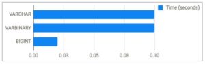
While optimizing query performance, we measured query speeds when using different data types for columnar indexes. We looked specifically at VARCHAR, VARBINARY, and BIGINT.
In our tests, we found that a numeric columnar index key data type (BIGINT) was faster than non-numeric (VARCHAR or VARBINARY). We measured BIGINT at ~0.02 seconds vs. five times longer for both non-numeric variations. Same data, same hardware, same queries. The only variable was changing the data type of the columnar index key. While the “slower” options were still quite fast, these findings were useful.
Execution Plans and the Plan Cache
SingleStore utilizes an embedded compiler to enable low-level optimizations that are unavailable via the standard interpreter-based database execution model. SingleStore uses these optimizations in query compilation. After a query is first run on each node, a compiled query and query plan are cached on disk for future use. All future occurrences of that query running will use the compiled query and execution plan. There are ways of writing your SQL that can work well in this regard, but it’s also possible to inadvertently write queries that have to be recompiled each time. Understanding how to look at the plan cache is useful. It’s also sometimes useful to manually remove a cached query if you’ve made changes and you want to try them out fresh.
Caches reset when nodes are restarted, which can be helpful (if you want to force reset everything in the cluster) or confusing (bounce a few nodes then wonder why things seem slow). The plan cache also has an expiration to it, so the cluster will periodically build new plans over time. We ran into this when our users would get back to the office on Monday morning — after a weekend of cluster inactivity — and discover that everything was slow. Once everything warmed up, performance would remain great through the week. With SingleStore’s guidance, we were able to tune the cache to accommodate this.
OR vs. IN
One of the scenarios we uncovered was using “OR” clauses as opposed to “IN” clauses in our SQL statements. Consider the following two queries:
Query A: SELECT * FROM foo WHERE id=1 OR id=2;
Query B: SELECT * FROM foo WHERE id=1 OR id=2 OR id=3;
As written, these will result in different execution plans even though the queries are very similar. In our usage, the “id=1 OR id=2” clause is dynamically generated, and could have anywhere from 1 to dozens or more OR statements. Since each slight variation results in a new execution plan, we ended up seeing intermittent slowness. This one took a while to identify.
It turns out there’s an easy fix — use IN clauses instead, like this:
Query A: SELECT * FROM foo WHERE id IN (1,2);
Query B: SELECT * FROM foo WHERE id IN (1,2,3);
Both of these queries (along with all other variations of numbers in the IN clause) land on the same execution plan, so they will all be fast.
Data Skew
Data skew occurs when data in a table is unevenly distributed across nodes in the cluster. SingleStore will distribute the data across the nodes using a shard key that you specify, or base it off the primary key if you don’t explicitly define one. A healthy distributed database should have approximately 1/N-th of your table data present on each of N nodes in your cluster. Measuring and observing data skew was useful to understand if we picked the best shard key.
Summary
When we started working on the new Ads dashboard in 2016, it wasn’t clear that we would be able to satisfy the project requirements. It was, after all, a challenging problem to solve. In fact, our initial research included me asking around to see how other large companies addressed this problem, and — without naming names — I found that several highly recognizable companies dealt with their ads dashboards much the same as we had already been doing (daily aggregation jobs that had problems and limitations). Surely, if this were easy to do, it would have already been done.
From the start it was very clear that we needed to pick a suitable data store or the entire project wouldn’t be a success. By focusing our options and narrowing down the field based on our requirements, we ended up choosing SingleStore. It fit very well with our project requirements, features, and performance needs. It’s also great that, a few years later, all of those have remained true.
As we built experience using SingleStore, we began looking for other data projects at Pandora that might be a good fit. In a few cases, there was a project that looked promising but a deeper dive showed things weren’t as good a fit after all (those projects either remained as is, or went a different, non-SingleStore direction). In other cases, we’ve found a great match between project needs and SingleStore’s strengths, so our usage of SingleStore has expanded beyond our initial Ads dashboard project.
The original posting of this blog can be found here.


